40 how to arrange row labels in pivot table

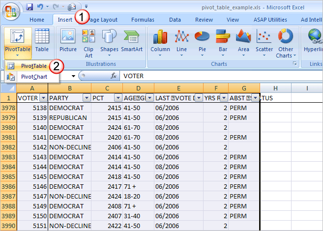
Sorting Row Labels in a Pivot Table by Month - Microsoft Community Sorting Row Labels in a Pivot Table by Month Hoping somebody can help please. I have a Dataset with dates people book holidays. I have a column using the =TEXT (A1,"mmm-yy") to get them grouped by month. I thine put that column in a pivot table but the table doesn't go from January -December. It does it by the first letter so April, Aug, Feb etc., How to add column labels in pivot table [SOLVED] Here are the steps. 1. Add a helper column showing Month Text Just as I have done in Column H. 2. Now insert a Pivot Table. 3. Put Fields in there required sections in the Pivot table Field List Window just as I have done . 4. Now Select the Row Lable column and Uncheck the Subtotal for Material field option.

Grouping, sorting, and filtering pivot data - Microsoft Press Store The pivot table in that figure is using Tabular layout. If your pivot tables use Compact layout, you see a drop-down menu on the cell with Row Labels or Column Labels. If you have multiple row fields, it is just as easy to sort using the invisible drop-down menus that appear when you hover over a field in the top of the PivotTable Fields list.

How to arrange row labels in pivot table

vba - Arrange pivot row labels in fixed order - Stack Overflow Get a given pivot item of the second row field given a particular pivot item in the first row field 0 I would like to create a very simple pivot table using vba, but I keep getting errors with my pivot cache Changing Order of Row Labels in Pivot Table - YouTube If the pivot table isn't properly sorting your row labels, you can bully it around to do what you want. This video shows you how How to rename group or row labels in Excel PivotTable? 1. Click at the PivotTable, then click Analyze tab and go to the Active Field textbox. 2. Now in the Active Field textbox, the active field name is displayed, you can change it in the textbox. You can change other Row Labels name by clicking the relative fields in the PivotTable, then rename it in the Active Field textbox.

How to arrange row labels in pivot table. Excel tutorial: How to rearrange fields in a pivot table In this pivot table, we have the Product field in the Row Labels area and Region in the Column Labels areas. We can just drag the fields to swap locations. And drag them back again to restore the original orientation. In this same way, we can look at product sales by region and state by adding State to the Column labels area. How to make row labels on same line in pivot table? 1. Click any one cell in the pivot table, and right click to choose PivotTable Options, see screenshot: 2. In the PivotTable Options dialog box, click the Display tab, and then check Classic PivotTable layout (enables... 3. Then click OK to close this dialog, and you will get the following pivot ... Sort multiple row label in pivot table - Microsoft Community Sort multiple row label in pivot table. Hi All. Could anybody suggest how to sort the pivot table row field data if it contains multiple headers :-. for example : In below given example I want to sort the data of column B in asending order , but when I am applying sorting here it is not sorting. Thanks in advance for your suggestion. Pivot Table Row Labels In the Same Line - Beat Excel! First make a pivot table with required fields. Arrange the fields as shown in left picture. Your initial table will look like right picture. Now click on "Error Code" and access field settings. First check "None" option in "Subtotals & Filters" tab to disable totals after every row.

Excel Pivot Tables - Sorting Data - Tutorials Point You can sort the data in the above PivotTable on Fields that are in Rows or Columns - Region, Salesperson and Month. To sort the PivotTable with the field Salesperson, proceed as follows −. Click the arrow in the Row Labels. Select Salesperson in the Select Field box from the dropdown list. More Sort Options. docs.devexpress.com › WindowsForms › 113894Get Started With Data Grid and Views - DevExpress Apr 04, 2022 · Displays records as read-only tiles, using one of the following layout modes: default (standard table layout), list (tiles have no space between them), and Kanban. This View includes the Tile Template feature, which helps you arrange fields relative to other fields, specify absolute or relative field display bounds, etc. Pivot table row labels in separate columns • AuditExcel.co.za So when you click in the Pivot Table and click on the DESIGN tab one of the options is the Report Layout. Click on this and change it to Tabular form. Your pivot table report will now look like the bottom picture and will be easier to use in other areas of the spreadsheet and in our opinion is also easier to read. › pivot-table › how-toHow to sort columns in pivot table in Excel | Basic Excel ... Sep 13, 2021 · With the selected data select the Insert tab and then press Pivot Tables. Then select From Table/Range. This will create the pivot table from the existing table you highlighted. Having created the PivotTable, the first step in sorting column data. We click the field with the data or items that need Sort. The option is at the Pivot table.

How to Customize Your Excel Pivot Chart Data Labels - dummies To add data labels, just select the command that corresponds to the location you want. To remove the labels, select the None command. If you want to specify what Excel should use for the data label, choose the More Data Labels Options command from the Data Labels menu. Excel displays the Format Data Labels pane. How to Sort Pivot Table Columns and Rows - EDUCBA First, we can click right the pivot table field we want to sort and select the appropriate option from the Sort by list. Also, we can choose More Sort Options from the same list to sort more. Another way is by applying the filter in a Pivot table. Go to the cell out of the table and press Shift + Ctrl + L together to apply the filter. How to Use Excel Pivot Table Label Filters Watch the steps in this short video, and the written instructions are below the video. Play. To change the Pivot Table option to allow multiple filters: Right-click a cell in the pivot table, and click PivotTable Options. Click the Totals & Filters tab Under Filters, add a check mark to 'Allow multiple filters per field.'. How to Move Excel Pivot Table Labels Quick Tricks Click on the cell where you want a different label to appear Type the name of the label that you want to move Press Enter The existing labels shift down, and the moved label takes its new position. For example, type "West" in cell A4, over the existing District name, "Central" Then, press Enter, to complete the change.

How To Create A Pivot Table With Multiple Columns And Rows | Cabinets Matttroy

superuser.com › questions › 1099503Creating a "grouped" bar chart from a table in Excel - Super User If you have a formula somewhere that relies on the whole column in a table, then if you add or remove rows in the table, the formula will update without any effort on your part. These formulas include the Series formulas in the chart. So add a row to the table, and the chart will automatically include the new row of data.

Excel Pivot Table Tutorial & Sample | Productivity Portfolio

docs.lvgl.io › master › overviewOverview — LVGL documentation A simple row and a column layout with flexbox; Arrange items in rows with wrap and even spacing; Demonstrate flex grow; Demonstrate flex grow. Demonstrate column and row gap style properties; RTL base direction changes order of the items; Grid. A simple grid; Demonstrate cell placement and span; Demonstrate grid's "free unit" Demonstrate track ...

How To Create A Pivot Table With Multiple Columns And Rows | Cabinets Matttroy

Sort data in a PivotTable or PivotChart Follow these steps to sort in Excel Desktop: In a PivotTable, click the small arrow next to Row Labels and Column Labels cells. Click a field in the row or column you want to sort. Click the arrow on Row Labels or Column Labels, and then click the sort option you want. To sort data in ascending or descending order, click Sort A to Z or Sort Z to A.

Pivot Table Row Labels In the Same Line - Beat Excel!

Pivot table row labels side by side - Excel Tutorials Now, let's create a pivot table ( Insert >> Tables >> Pivot Table) and check all the values in Pivot Table Fields. Fields should look like this. Right-click inside a pivot table and choose PivotTable Options…. Check data as shown on the image below. The table is going to change. The pivot table is almost ready.

Arrange Value Fields Vertically for Printing – Excel Pivot Tables

cdn.ablebits.com › _img-docs › ultimate-suiteUltimate Suite for Excel Comprehensive set of time-saving ... 1.Use Unpivot Table to transform your pivot table (crosstab) to a one-dimensional list and save the result to another worksheet or workbook, without corrupting the original data. 2.Run Create Cards to turn your table data into label cards – address or mailing labels, price tags and other kinds of cards.

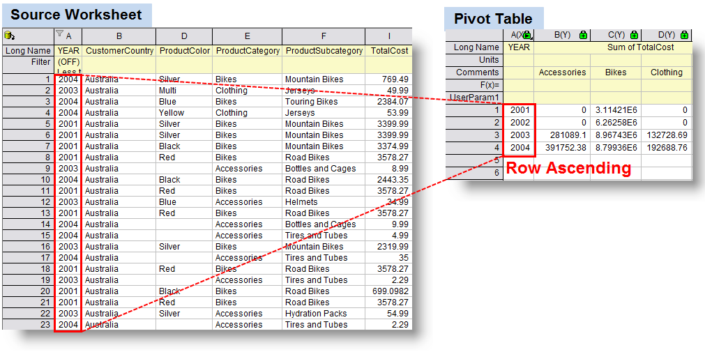
Help Online - Origin Help - Pivot Table

Sorting to your Pivot table row labels in custom order [quick tip] Using MATCH formula, find the order of each row label (in our case, classification) in the sort order list. Assuming classification is in D3, use =MATCH (D3, $I$3:$I$12, 0) Create a pivot table with data set including sort order column. Add sort order column along with classification to the pivot table row labels area.

Excel Master Series Blog: Simplifying Excel Pivot Table and Pivot Chart Setup

How do I have multiple row labels in a pivot table? Activate the pivot table. Select the first cell and then use Shift+click to include a contiguous group of cells or Ctrl+click (Command+click on Mac) to select additional cells one at a time. Activate the pivot table. Click a row or column label. Click the row or column label again.

Arrange Pivot Table Data Vertically – Excel Pivot Tables

How to Add Rows to a Pivot Table: 9 Steps (with Pictures) Click anywhere in your pivot table. This opens the pivot table editor on the right side of Google Sheets. 3. Click Add under "Rows." It's in the left side of the pivot table editor. A list of fields will expand on the menu. 4. Click the name of the field you want to add as a row.

Share :